Large language models are usually treated as a black box: a prompt goes in, text comes out, and whatever happens in between stays inside. LLM-Scope opens that box on a model that's real but small enough to run on any computer — Qwen3-0.6B, 28 layers.
The app shows every number that gets computed along the way: neuron activations, attention weights, intermediate predictions at every depth, and the complete path a single token takes through the network.
Static demo: mpiotro4.github.io/LLM-Scope
source code: github.com/mpiotro4/LLM-Scope.
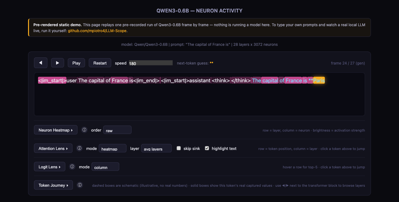
Every panel is independently collapsible and has its own ⓘ button with a longer explanation — the rest of this write-up doubles as a walkthrough you can click through yourself in the demo.
How you actually use it
You type a prompt, the model generates a response, and the app replays the whole thing as frames — one frame per token. You can step through them, hit play to watch it animate, and adjust the speed; first comes the prompt-reading phase, then token-by-token generation.
The key part is that every panel shares one selection. Clicking any token in the text moves the heatmap, attention, logit lens and Token Journey to that same position at once, so you're always looking at a single moment of computation from four different angles.
Neuron activation heatmap
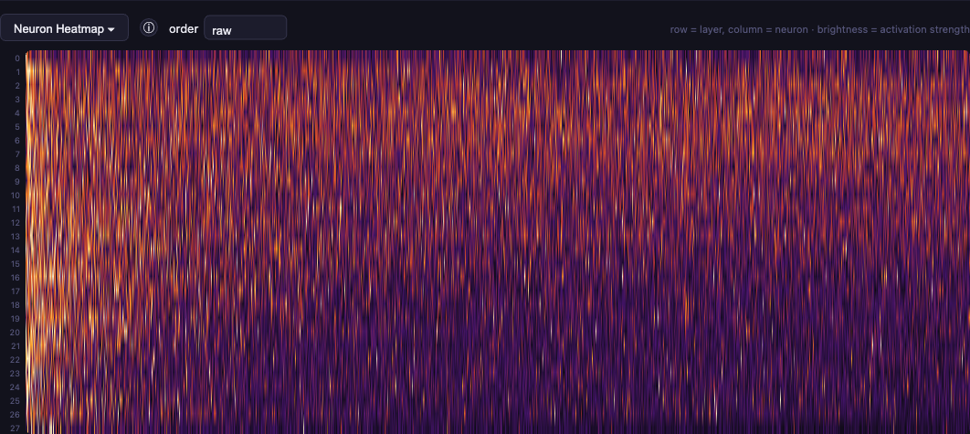
The model has 28 layers, and each one ends its computation with a wide feed-forward network (a SwiGLU MLP) of 3072 "neurons." The heatmap shows how strongly each one fired for the currently selected token — row = layer, column = neuron, brightness = |activation|.
Two things had to be solved to make this actually legible:
- Scale. A handful of neurons in every layer can have values an order of magnitude larger than the rest ("massive activations" — a well-documented phenomenon in large models). Normalizing by the maximum would crush everything else to black. Instead, each layer is clipped to its own 99th percentile and additionally sqrt-compressed, squeezing the dynamic range without losing the weaker signal.
- Neuron order. MLP hidden units have no inherent ordering (permutation symmetry) — the model's native order is visually pure noise.
compute_neuron_order.pycomputes a stable order once, offline, via correlation-based hierarchical clustering over a diverse prompt corpus, so correlated neurons end up next to each other. In the UI this is theorderselector:raw,clusteredorby mean.
Worth saying up front what this heatmap doesn't do: with 3072 columns squeezed into the window width, a single neuron occupies a fraction of a pixel, so you can't read anything off it. It's purely a visualization of scale. Every one of these neurons carries a carefully learned weight, the product of expensive training — which makes it all the more striking that the large models we use every day have 100 times as many.
Attention
Clicking any token in the text washes earlier tokens in pink, proportional to how much attention that token paid them (averaged over all 16 attention heads, or for a single chosen layer). The Attention Lens panel below shows the same row at full resolution: row = earlier token, column = layer (0–27), brightness = attention weight.
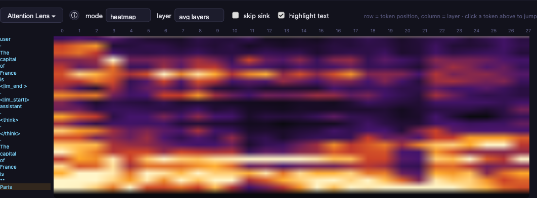
An implementation detail worth calling out: why exactly one cell per layer, rather than one per head? Because the 16 heads are averaged together at capture time, on the Python side, before anything reaches the data sent to the browser. For a given layer there is therefore exactly one number per earlier token, and per-head resolution is thrown away irreversibly at that stage — the front-end never sees it. For the same reason, the layer selector has no effect on heatmap mode, which always shows all 28 layers at once; it only matters in column mode and for the text overlay.
A second quirk: the very first token in a sequence routinely soaks up a disproportionate share of attention at every layer — the well-documented "attention sink" phenomenon. Left in as a reference point it would crush the rest of the scale to near-invisible, so it's excluded from normalization while still rendering at full intensity itself. The skip sink checkbox hides it from the panel entirely and rescales against what's left, and the difference is dramatic: while generating "Paris", everything looks uniformly dark without it; turn it on and you can see the model attending mainly to "France" and "capital" — exactly where it should be looking.
Seeing attention at all requires weights the fast default kernel (sdpa) never computes explicitly — the model has to be loaded with attn_implementation="eager" instead, which costs roughly 8–9x more time per token.
Logit lens
At every depth — the embedding output ("layer -1") and the output of each of the 28 transformer blocks — the residual stream is projected through the model's own final norm and lm_head, as if the network had stopped computing right there. It's a way to eavesdrop on what the model "believes" long before it's actually done.
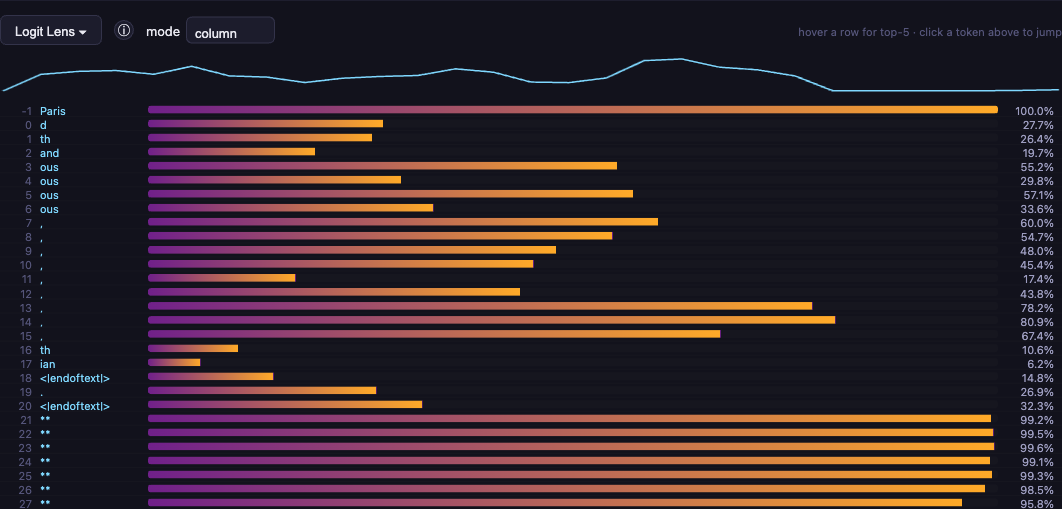
For intermediate layers this is only an approximation: the residual stream isn't expressed in the basis lm_head operates in until the final layer, so projecting earlier depths through that same matrix is a heuristic, not something the model was trained to support.
In practice you see exactly that pattern. For the prompt "The capital of France is", the prediction following "Paris" is essentially random for the first twenty layers — fragments like "ous" or a comma show up — and then from layer 21 it locks onto ** (closing the bold) at 96–99% confidence and never moves again. Watching exactly where that moment happens is interesting in its own right.
There's one more artifact right at the top of the list: at depth -1, just after the embedding, the model "predicts" the very token it's currently reading. That's not a bug — Qwen3 ties the embedding and lm_head weights (lm_head.weight is literally the same tensor as embed_tokens.weight), so projecting a fresh embedding back through that matrix lands hardest on the token itself.
Generation is greedy — plain argmax, no sampling. That's deliberate: it means the deepest logit-lens row performs exactly the same computation the model does, and matches its output bit for bit. Sampling would add noise that muddies the very thing this panel exists to show.
Token Journey
A panel that walks the single, currently-selected token through the whole pipeline, top to bottom: tokenization (text → vocabulary ID) → embedding vector → the internals of one transformer block (with its own layer stepper, independent of every other panel) → output vector → prediction → detokenization.
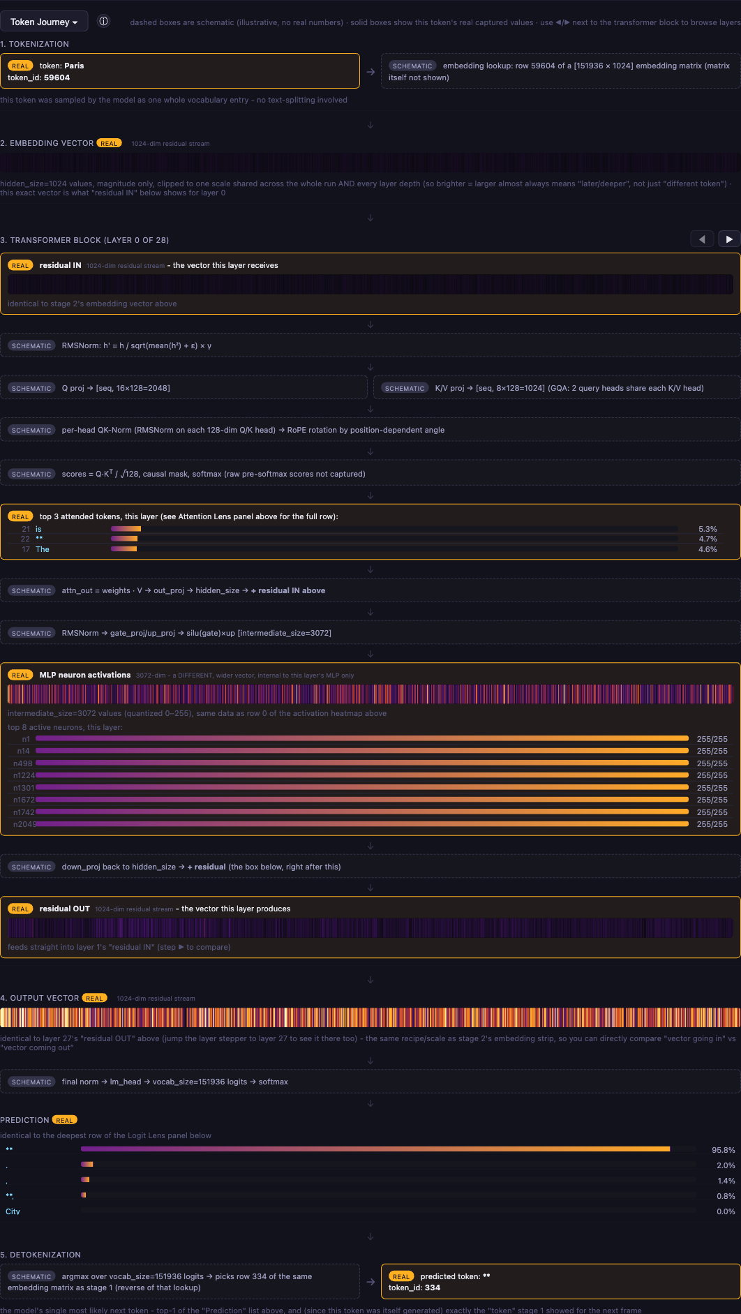
The whole panel follows one rule: it never shows a number it didn't capture. Solid amber boxes hold this token's actual values — the same numbers as the panels above, plus the embedding, residual and output vectors themselves as small heatmap strips. Dashed boxes are schematics of what the app never records or transmits: raw Q/K/V vectors, RoPE angles, pre-softmax scores. You get the formula and the tensor shape, never an invented number.
One detail that's easy to miss and that the panel gets right: in Qwen3 the per-head dimension (128) does not come from dividing hidden_size by the head count, which would give 1024/16 = 64. The Q projection therefore comes out wider than the residual stream itself — 16 × 128 = 2048 against 1024. Most transformer explainers quietly assume that division and print the wrong shapes.
The 1024-dim vector shown as "residual IN", "residual OUT", the embedding vector and the output vector is the same running quantity at every stage — one layer's OUT is identical to the next layer's IN, all the way from the embedding lookup to the final output vector. Stepping through layers with the transformer block's own arrows shows this single vector gradually deforming as it passes through all 28 layers.
Two modes: offline and live
All the capture logic (model loading, hooks, the generation loop, the logit lens) lives in one module shared by two independent entry points:
- Offline replay (
capture.py) — runs one prompt through the model and writes the whole run out as a single self-contained HTML file you can open offline and scrub through frame by frame. The shared CSS/JS fromstatic/is inlined directly into the file, so the output is one dependency-free file — this is exactly the file that ends up on GitHub Pages. - Live (
server.py) — keeps the model resident in memory and streams activity over Server-Sent Events as you type prompts. One model instance serves one request at a time (a simple global lock) — fine for local use, not for concurrent multi-user hosting.
Deployment and CI/CD
The static demo is automatically built by a GitHub Action rather than being a manually refreshed snapshot. On every push to main, the pipeline installs dependencies, downloads and caches Qwen3-0.6B (~1.2 GB, once), runs capture.py on a CI runner, and publishes the resulting HTML to GitHub Pages through the official actions/deploy-pages action. Nothing is committed back — the generated file lives only as the Pages deployment, so the git history doesn't accumulate yet another copy of the same multi-megabyte file on every refresh.
Tech stack
- PyTorch + Transformers (
AutoModelForCausalLM/AutoTokenizer) — model loading, forward hooks on every layer'sdown_proj(capturing MLP activations) and on each block's output (capturing the residual stream) - FastAPI + Server-Sent Events — the live mode
- Plain JavaScript + Canvas, no framework — a deliberate choice so the offline output can stay a single HTML file with no build step
- NumPy / SciPy / Pillow — neuron-order clustering and the verification script
- pytest — the test suite, including a golden test that catches the numeric pipeline quietly starting to return something different
- GitHub Actions — CI/CD to GitHub Pages
Limitations
- Attention requires
attn_implementation="eager", roughly 8–9x slower than the default fast kernel — the cost of extracting weights the model never normally materializes explicitly. - The logit lens is a heuristic for intermediate layers, not a strict interpretation (see above) — only the deepest layer is guaranteed to match the model's actual prediction.
- The heatmap squeezes 3072 columns into the window width, so you can't read an individual neuron off it — it shows the pattern, not the specifics.
- Attention weights are averaged over heads at capture time, so per-head structure isn't available.
- A hard cap of 300 new tokens (the model usually hits EOS well before that anyway) — each frame carries a heavy payload (activations + attention + logit lens), so an open-ended limit would risk a multi-gigabyte HTML file or a very long stream.
server.pyserves one generation request at a time — this is not multi-user hosting.- Neuron order in the heatmap is arbitrary until
compute_neuron_order.pyhas been run once. - This is a tool for observation, not intervention — you can't silence a neuron or clamp attention and watch the output change.